Optimal POVM

One can open this tutorial in Google Colab (is recommended)

In the following tutorial, we show how to perform optimization over the manifold of POVMs by using the QGOpt library. It is known that measurements of a qubit induced by tetrahedral POVM allow reconstructing an unknown qubit state with a minimal variance if there is no prior information about a qubit state. Let us check this fact numerically using optimization over the manifold of POVMs. In the beginning, let us import some libraries.

import tensorflow as tf  # tf 2.x
import matplotlib.pyplot as plt
import math

try:
    import QGOpt as qgo
except ImportError:
    !pip install git+https://github.com/LuchnikovI/QGOpt@Dev
    import QGOpt as qgo

# Fix random seed to make results reproducable.
tf.random.set_seed(42)

1. Prior information about a quantum state

We represent a prior probability distribution over a quantum state approximately, by using a set of samples from a prior distribution. Since tetrahedral POVM is optimal when there is no prior information about a state, we consider uniform distribution across the Bloch ball.

#-------------------------------------------------------------------------#
num_of_samples = 10000  # number of samples representing prior information
#-------------------------------------------------------------------------#

# Pauli matrices
sigma_x = tf.constant([[0, 1], [1, 0]], dtype=tf.complex128)
sigma_y = tf.constant([[0 + 0j, -1j], [1j, 0 + 0j]], dtype=tf.complex128)
sigma_z = tf.constant([[1, 0], [0, -1]], dtype=tf.complex128)

# All Pauli matrices in one tensor of shape (3, 2, 2)
sigma = tf.concat([sigma_x[tf.newaxis],
                   sigma_y[tf.newaxis],
                   sigma_z[tf.newaxis]], axis=0)

# Set of points distributed uniformly across Bloch ball
x = tf.random.normal((num_of_samples, 3), dtype=tf.float64)
x = x / tf.linalg.norm(x, axis=-1, keepdims=True)
x = tf.cast(x, dtype=tf.complex128)
u = tf.random.uniform((num_of_samples, 1), maxval=1, dtype=tf.float64)
u = u ** (1 / 3)
u = tf.cast(u, dtype=tf.complex128)
x = x * u

# Set of density matrices distributed uniformly across Bloch ball
# (prior information)
rho = 0.5 * (tf.eye(2, dtype=tf.complex128) + tf.tensordot(x, sigma, axes=1))

2. Search for the optimal POVM with given prior information about a state

Here we search for the optimal POVM via minimizing the variance of a posterior distribution over density matrices. First, we define an example of the POVMs manifold:

m = qgo.manifolds.POVM()

The manifolds of POVMs is represented through the quadratic parametrization \(M_i = A_iA_i^\dagger\) with an equivalence relation \(A_i\sim A_iQ_i\), where \(Q_i\) is an arbitrary unitary matrix. Here, we initialize a variable that represents the parametrization of each element of POVM:

# randon initial parametrization of POVM
A = m.random((4, 2, 2), dtype=tf.complex128)
# real representtion of A
A = qgo.manifolds.complex_to_real(A)
# tf.Variable to be tuned
A = tf.Variable(A)

Then we initialize Riemannian Adam optimizer:

lr = 0.03
opt = qgo.optimizers.RAdam(m, lr)

Finally, we ran the part of code that calculates forward pass, gradients, and optimization step several times until convergence to the optimal point is reached:

for i in range(1000):
    with tf.GradientTape() as tape:

        # Complex representation of A
        Ac = qgo.manifolds.real_to_complex(A)
        # POVM from its parametrization
        povm = Ac @ tf.linalg.adjoint(Ac)
        # Inverce POVM (is needed to map a probability distribution to a density matrix)
        povm_inv = tf.linalg.inv(tf.reshape(povm, (4, 4)))
        # Matrix T maps probability vector to four real parameters representing
        # a quantum state (equivalent to inverse POVM)
        T = tf.concat([tf.math.real(povm_inv[0, tf.newaxis]),
                        tf.math.real(povm_inv[3, tf.newaxis]),
                        tf.math.real(povm_inv[2, tf.newaxis]),
                        tf.math.imag(povm_inv[2, tf.newaxis])], axis=0)

        # POVM maps a quantum state to a probability vector
        p = tf.tensordot(rho, povm, axes=[[2], [1]])
        p = tf.transpose(p, (0, 2, 1, 3))
        p = tf.math.real(tf.linalg.trace(p))

        # Covariance matrix of a reconstructed density matrix
        cov = -p[:, tf.newaxis] * p[..., tf.newaxis]
        cov = cov + tf.linalg.diag(p ** 2)
        cov = cov + tf.linalg.diag(p * (1 - p))
        cov = tf.tensordot(T, cov, [[1], [1]])
        cov = tf.tensordot(cov, T, [[2], [1]])
        cov = tf.transpose(cov, (1, 0, 2))

        # Covariance matrix avaraged over prior distribution
        av_cov = tf.reduce_mean(cov, axis=0)

        # loss function (log volume of Covariance matrix)
        loss = tf.reduce_sum(tf.math.log(tf.linalg.svd(av_cov)[0][:-1]))
    grad = tape.gradient(loss, A)  # gradient
    opt.apply_gradients(zip([grad], [A]))  # minimization step

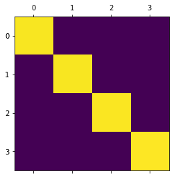
3. Verification

Here we check the resulting optimal POVM. For tetrahedral POVM one has the following relation \({\rm Tr}\left(M^\alpha M^\beta\right) = \frac{2\delta_{\alpha\beta} + 1}{12}\). One can see, that this relation is almost true for a resulting POVM. The small error appears due to the approximate Monte-Carlo averaging of a covariance matric by using a set of samples from the prior distribution.

cross = tf.tensordot(povm, povm, [[2], [1]])
cross = tf.transpose(cross, (0, 2, 1, 3))
cross = tf.linalg.trace(cross)
cross = tf.math.real(cross)
plt.matshow(cross)
print(cross)

tf.Tensor(
[[0.24927765 0.08337808 0.08333673 0.08328467]
 [0.08337808 0.24939711 0.08328523 0.08333633]
 [0.08333673 0.08328523 0.25029829 0.08337795]
 [0.08328467 0.08333633 0.08337795 0.25102899]], shape=(4, 4), dtype=float64)